今すぐ見るこのチュートリアルには、RealPythonチームによって作成された関連するビデオコースがあります。理解を深めるために、書かれたチュートリアルと一緒にそれを見てください:パンダでファイルを読んだり書いたりする
パンダ は強力で柔軟なPythonパッケージであり、ラベル付きの時系列データを操作できます。また、統計手法を提供し、プロットなどを可能にします。 Pandasの重要な機能の1つは、Excel、CSV、およびその他の多くの種類のファイルを読み書きできることです。パンダのような機能read_csv() メソッドを使用すると、ファイルを効果的に操作できます。それらを使用して、Pandasオブジェクトのデータとラベルをファイルに保存し、後でPandasシリーズとしてロードできます。 またはDataFrame インスタンス。
このチュートリアルでは、次のことを学びます。
- PandasIOツールとは APIは
- データの読み取りと書き込みの方法 ファイルとの間
- さまざまなファイル形式を操作する方法
- ビッグデータの操作方法 効率的に
ファイルの読み取りと書き込みを始めましょう!
パンダのインストール
このチュートリアルのコードは、CPython3.7.4およびPandas0.25.1で実行されます。マシンに最新バージョンのPythonとPandasがあることを確認すると便利です。新しい仮想環境を作成し、このチュートリアルの依存関係をインストールすることをお勧めします。
まず、Pandasライブラリが必要です。すでにインストールされている可能性があります。そうでない場合は、pipを使用してインストールできます:
$ pip install pandas
インストールプロセスが完了したら、Pandasをインストールして準備ができているはずです。
アナコンダ は、Python、Pandasなどの多くの便利なパッケージ、およびCondaと呼ばれるパッケージおよび環境マネージャーが付属する優れたPythonディストリビューションです。 Anacondaの詳細については、Windowsでの機械学習用のPythonの設定をご覧ください。
仮想環境にパンダがない場合は、Condaを使用してインストールできます:
$ conda install pandas
Condaは、依存関係とそのバージョンを管理するため、強力です。 Condaの操作について詳しくは、公式ドキュメントをご覧ください。
データの準備
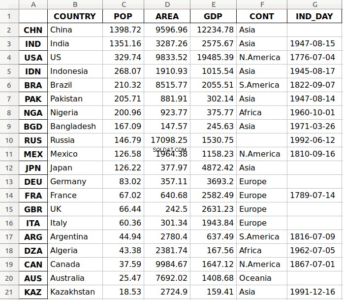
このチュートリアルでは、20か国に関連するデータを使用します。使用するデータとソースの概要は次のとおりです。
-
国 国名で示されます。各国は、人口、地域、または国内総生産(GDP)のいずれかでトップ10リストに含まれています。データセットの行ラベルは、ISO3166-1で定義されている3文字の国コードです。データセットの列ラベルは
COUNTRYです。 。 -
人口 百万で表されます。データは、ウィキペディアの人口別の国と依存関係のリストから取得されます。データセットの列ラベルは
POPです。 。 -
エリア 数千平方キロメートルで表されます。データは、ウィキペディアの地域別の国と依存関係のリストから取得されます。データセットの列ラベルは
AREAです。 。 -
国内総生産 2017年の国連のデータによると、は数百万米ドルで表されます。このデータは、ウィキペディアの名目GDP別の国のリストにあります。データセットの列ラベルは
GDPです。 。 -
大陸 アフリカ、アジア、オセアニア、ヨーロッパ、北アメリカ、または南アメリカのいずれかです。この情報はウィキペディアでも見つけることができます。データセットの列ラベルは
CONTです。 。 -
独立記念日 国の独立を記念する日付です。データは、ウィキペディアの全国独立日のリストからのものです。日付はISO8601形式で表示されます。最初の4桁は年を表し、次の2桁は月を表し、最後の2桁は月の日を表します。データセットの列ラベルは
IND_DAYです。 。
これは、データがテーブルとしてどのように見えるかです:
| 国 | POP | エリア | GDP | 続き | IND_DAY | |
|---|---|---|---|---|---|---|
| CHN | 1398.72 | 9596.96 | 12234.78 | |||
| IND | 1351.16 | 3287.26 | 2575.67 | 1947-08-15 | ||
| 米国 | 329.74 | 9833.52 | 19485.39 | 1776-07-04 | ||
| IDN | 268.07 | 1910.93 | 1015.54 | 1945-08-17 | ||
| BRA | 210.32 | 8515.77 | 2055.51 | S.America | 1822-09-07 | |
| PAK | 205.71 | 881.91 | 302.14 | 1947-08-14 | ||
| NGA | 200.96 | 923.77 | 375.77 | 1960-10-01 | ||
| BGD | 167.09 | 147.57 | 245.63 | 1971-03-26 | ||
| RUS | 146.79 | 17098.25 | 1530.75 | 1992-06-12 | ||
| MEX | 126.58 | 1964.38 | 1158.23 | 1810-09-16 | ||
| JPN | 126.22 | 377.97 | 4872.42 | |||
| DEU | 83.02 | 357.11 | 3693.20 | |||
| FRA | 67.02 | 640.68 | 2582.49 | 1789-07-14 | ||
| GBR | 66.44 | 242.50 | 2631.23 | |||
| ITA | 60.36 | 301.34 | 1943.84 | |||
| ARG | 44.94 | 2780.40 | 637.49 | S.America | 1816-07-09 | |
| DZA | 43.38 | 2381.74 | 167.56 | 1962-07-05 | ||
| CAN | 37.59 | 9984.67 | 1647.12 | 1867-07-01 | ||
| AUS | 25.47 | 7692.02 | 1408.68 | |||
| KAZ | 18.53 | 2724.90 | 159.41 | 1991-12-16 |
一部のデータが欠落していることに気付くかもしれません。たとえば、ロシア大陸はヨーロッパとアジアの両方に広がっているため、指定されていません。データソースで独立日が省略されているため、独立日が欠落している日もいくつかあります。
ネストされた辞書を使用して、Pythonでこのデータを整理できます:
data = {
    'CHN': {'COUNTRY': 'China', 'POP': 1_398.72, 'AREA': 9_596.96,
            'GDP': 12_234.78, 'CONT': 'Asia'},
    'IND': {'COUNTRY': 'India', 'POP': 1_351.16, 'AREA': 3_287.26,
            'GDP': 2_575.67, 'CONT': 'Asia', 'IND_DAY': '1947-08-15'},
    'USA': {'COUNTRY': 'US', 'POP': 329.74, 'AREA': 9_833.52,
            'GDP': 19_485.39, 'CONT': 'N.America',
            'IND_DAY': '1776-07-04'},
    'IDN': {'COUNTRY': 'Indonesia', 'POP': 268.07, 'AREA': 1_910.93,
            'GDP': 1_015.54, 'CONT': 'Asia', 'IND_DAY': '1945-08-17'},
    'BRA': {'COUNTRY': 'Brazil', 'POP': 210.32, 'AREA': 8_515.77,
            'GDP': 2_055.51, 'CONT': 'S.America', 'IND_DAY': '1822-09-07'},
    'PAK': {'COUNTRY': 'Pakistan', 'POP': 205.71, 'AREA': 881.91,
            'GDP': 302.14, 'CONT': 'Asia', 'IND_DAY': '1947-08-14'},
    'NGA': {'COUNTRY': 'Nigeria', 'POP': 200.96, 'AREA': 923.77,
            'GDP': 375.77, 'CONT': 'Africa', 'IND_DAY': '1960-10-01'},
    'BGD': {'COUNTRY': 'Bangladesh', 'POP': 167.09, 'AREA': 147.57,
            'GDP': 245.63, 'CONT': 'Asia', 'IND_DAY': '1971-03-26'},
    'RUS': {'COUNTRY': 'Russia', 'POP': 146.79, 'AREA': 17_098.25,
            'GDP': 1_530.75, 'IND_DAY': '1992-06-12'},
    'MEX': {'COUNTRY': 'Mexico', 'POP': 126.58, 'AREA': 1_964.38,
            'GDP': 1_158.23, 'CONT': 'N.America', 'IND_DAY': '1810-09-16'},
    'JPN': {'COUNTRY': 'Japan', 'POP': 126.22, 'AREA': 377.97,
            'GDP': 4_872.42, 'CONT': 'Asia'},
    'DEU': {'COUNTRY': 'Germany', 'POP': 83.02, 'AREA': 357.11,
            'GDP': 3_693.20, 'CONT': 'Europe'},
    'FRA': {'COUNTRY': 'France', 'POP': 67.02, 'AREA': 640.68,
            'GDP': 2_582.49, 'CONT': 'Europe', 'IND_DAY': '1789-07-14'},
    'GBR': {'COUNTRY': 'UK', 'POP': 66.44, 'AREA': 242.50,
            'GDP': 2_631.23, 'CONT': 'Europe'},
    'ITA': {'COUNTRY': 'Italy', 'POP': 60.36, 'AREA': 301.34,
            'GDP': 1_943.84, 'CONT': 'Europe'},
    'ARG': {'COUNTRY': 'Argentina', 'POP': 44.94, 'AREA': 2_780.40,
            'GDP': 637.49, 'CONT': 'S.America', 'IND_DAY': '1816-07-09'},
    'DZA': {'COUNTRY': 'Algeria', 'POP': 43.38, 'AREA': 2_381.74,
            'GDP': 167.56, 'CONT': 'Africa', 'IND_DAY': '1962-07-05'},
    'CAN': {'COUNTRY': 'Canada', 'POP': 37.59, 'AREA': 9_984.67,
            'GDP': 1_647.12, 'CONT': 'N.America', 'IND_DAY': '1867-07-01'},
    'AUS': {'COUNTRY': 'Australia', 'POP': 25.47, 'AREA': 7_692.02,
            'GDP': 1_408.68, 'CONT': 'Oceania'},
    'KAZ': {'COUNTRY': 'Kazakhstan', 'POP': 18.53, 'AREA': 2_724.90,
            'GDP': 159.41, 'CONT': 'Asia', 'IND_DAY': '1991-12-16'}
}

columns = ('COUNTRY', 'POP', 'AREA', 'GDP', 'CONT', 'IND_DAY')
テーブルの各行は、キーが列名であり、値が対応するデータである内部ディクショナリとして書き込まれます。これらのディクショナリは、外部の dataの値として収集されます。 辞書。 dataに対応するキー は3文字の国コードです。
このdataを使用できます パンダのインスタンスを作成するにはDataFrame 。まず、パンダをインポートする必要があります:
>>> import pandas as pd
パンダをインポートしたので、 DataFrameを使用できます。 コンストラクターとdata DataFrameを作成するには オブジェクト。
データ 国コードが列に対応するように編成されています。 DataFrameの行と列を逆にすることができます プロパティ.Tを使用します :
>>> df = pd.DataFrame(data=data).T
>>> df
        COUNTRY      POP     AREA      GDP       CONT     IND_DAY
CHN       China  1398.72  9596.96  12234.8       Asia         NaN
IND       India  1351.16  3287.26  2575.67       Asia  1947-08-15
USA          US   329.74  9833.52  19485.4  N.America  1776-07-04
IDN   Indonesia   268.07  1910.93  1015.54       Asia  1945-08-17
BRA      Brazil   210.32  8515.77  2055.51  S.America  1822-09-07
PAK    Pakistan   205.71   881.91   302.14       Asia  1947-08-14
NGA     Nigeria   200.96   923.77   375.77     Africa  1960-10-01
BGD  Bangladesh   167.09   147.57   245.63       Asia  1971-03-26
RUS      Russia   146.79  17098.2  1530.75        NaN  1992-06-12
MEX      Mexico   126.58  1964.38  1158.23  N.America  1810-09-16
JPN       Japan   126.22   377.97  4872.42       Asia         NaN
DEU     Germany    83.02   357.11   3693.2     Europe         NaN
FRA      France    67.02   640.68  2582.49     Europe  1789-07-14
GBR          UK    66.44    242.5  2631.23     Europe         NaN
ITA       Italy    60.36   301.34  1943.84     Europe         NaN
ARG   Argentina    44.94   2780.4   637.49  S.America  1816-07-09
DZA     Algeria    43.38  2381.74   167.56     Africa  1962-07-05
CAN      Canada    37.59  9984.67  1647.12  N.America  1867-07-01
AUS   Australia    25.47  7692.02  1408.68    Oceania         NaN
KAZ  Kazakhstan    18.53   2724.9   159.41       Asia  1991-12-16
これで、 DataFrameができました。 各国に関するデータが入力されたオブジェクト。
注: .transpose()を使用できます .Tの代わりに データセットの行と列を逆にします。 .transpose()を使用する場合 、次にオプションのパラメータ copyを設定できます 基になるデータをコピーするかどうかを指定します。デフォルトの動作はFalseです。 。
3.6より古いバージョンのPythonは、辞書内のキーの順序を保証しませんでした。古いバージョンのPythonとPandasで列の順序が維持されるようにするには、 index =columnsを指定できます。 :
>>> df = pd.DataFrame(data=data, index=columns).T
データの準備ができたので、ファイルの操作を開始する準備が整いました。
パンダの使用read_csv() および.to_csv() 機能
カンマ区切り値(CSV)ファイルは、 .csvを含むプレーンテキストファイルです。 表形式のデータを保持する拡張機能。これは、大量のデータを保存するための最も一般的なファイル形式の1つです。 CSVファイルの各行は、単一のテーブル行を表します。同じ行の値は、デフォルトではコンマで区切られていますが、区切り文字をセミコロン、タブ、スペース、またはその他の文字に変更できます。
CSVファイルを作成する
パンダのDataFrameを保存できます .to_csv()を含むCSVファイルとして :
>>> df.to_csv('data.csv')
それでおしまい!ファイルdata.csvを作成しました 現在の作業ディレクトリにあります。以下のコードブロックを展開して、CSVファイルがどのように表示されるかを確認できます。
,COUNTRY,POP,AREA,GDP,CONT,IND_DAY
CHN,China,1398.72,9596.96,12234.78,Asia,
IND,India,1351.16,3287.26,2575.67,Asia,1947-08-15
USA,US,329.74,9833.52,19485.39,N.America,1776-07-04
IDN,Indonesia,268.07,1910.93,1015.54,Asia,1945-08-17
BRA,Brazil,210.32,8515.77,2055.51,S.America,1822-09-07
PAK,Pakistan,205.71,881.91,302.14,Asia,1947-08-14
NGA,Nigeria,200.96,923.77,375.77,Africa,1960-10-01
BGD,Bangladesh,167.09,147.57,245.63,Asia,1971-03-26
RUS,Russia,146.79,17098.25,1530.75,,1992-06-12
MEX,Mexico,126.58,1964.38,1158.23,N.America,1810-09-16
JPN,Japan,126.22,377.97,4872.42,Asia,
DEU,Germany,83.02,357.11,3693.2,Europe,
FRA,France,67.02,640.68,2582.49,Europe,1789-07-14
GBR,UK,66.44,242.5,2631.23,Europe,
ITA,Italy,60.36,301.34,1943.84,Europe,
ARG,Argentina,44.94,2780.4,637.49,S.America,1816-07-09
DZA,Algeria,43.38,2381.74,167.56,Africa,1962-07-05
CAN,Canada,37.59,9984.67,1647.12,N.America,1867-07-01
AUS,Australia,25.47,7692.02,1408.68,Oceania,
KAZ,Kazakhstan,18.53,2724.9,159.41,Asia,1991-12-16
このテキストファイルには、カンマで区切られたデータが含まれています 。最初の列には行ラベルが含まれています。場合によっては、それらが無関係であることがわかります。それらを保持したくない場合は、引数 index =Falseを渡すことができます。 .to_csv()へ 。
CSVファイルを読む
データがCSVファイルに保存されたら、そのデータを時々読み込んで使用することをお勧めします。あなたはパンダのread_csv()でそれを行うことができます 機能:
>>> df = pd.read_csv('data.csv', index_col=0)
>>> df
        COUNTRY      POP      AREA       GDP       CONT     IND_DAY
CHN       China  1398.72   9596.96  12234.78       Asia         NaN
IND       India  1351.16   3287.26   2575.67       Asia  1947-08-15
USA          US   329.74   9833.52  19485.39  N.America  1776-07-04
IDN   Indonesia   268.07   1910.93   1015.54       Asia  1945-08-17
BRA      Brazil   210.32   8515.77   2055.51  S.America  1822-09-07
PAK    Pakistan   205.71    881.91    302.14       Asia  1947-08-14
NGA     Nigeria   200.96    923.77    375.77     Africa  1960-10-01
BGD  Bangladesh   167.09    147.57    245.63       Asia  1971-03-26
RUS      Russia   146.79  17098.25   1530.75        NaN  1992-06-12
MEX      Mexico   126.58   1964.38   1158.23  N.America  1810-09-16
JPN       Japan   126.22    377.97   4872.42       Asia         NaN
DEU     Germany    83.02    357.11   3693.20     Europe         NaN
FRA      France    67.02    640.68   2582.49     Europe  1789-07-14
GBR          UK    66.44    242.50   2631.23     Europe         NaN
ITA       Italy    60.36    301.34   1943.84     Europe         NaN
ARG   Argentina    44.94   2780.40    637.49  S.America  1816-07-09
DZA     Algeria    43.38   2381.74    167.56     Africa  1962-07-05
CAN      Canada    37.59   9984.67   1647.12  N.America  1867-07-01
AUS   Australia    25.47   7692.02   1408.68    Oceania         NaN
KAZ  Kazakhstan    18.53   2724.90    159.41       Asia  1991-12-16
この場合、パンダの read_csv() 関数は新しいDataFrameを返します ファイルdata.csvのデータとラベルを使用 、最初の引数で指定しました。この文字列は、URLを含む任意の有効なパスにすることができます。
パラメータindex_col 行ラベルを含むCSVファイルの列を指定します。このパラメーターには、ゼロベースの列インデックスを割り当てます。 index_colの値を決定する必要があります CSVファイルに行ラベルが含まれている場合。データとしてのロードを回避します。
このチュートリアルの後半で、CSVファイルでのPandasの使用について詳しく学習します。 PythonでのCSVファイルの読み取りと書き込みをチェックして、組み込みのPythonライブラリcsvを使用してCSVファイルを処理する方法を確認することもできます。
パンダを使用したExcelファイルの書き込みと読み取り
Microsoft Excelは、おそらく最も広く使用されているスプレッドシートソフトウェアです。古いバージョンではバイナリ.xlsが使用されていました ファイル、Excel2007は新しいXMLベースの.xlsxを導入しました ファイル。 CSVファイルと同様に、PandasでExcelファイルを読み書きできます。ただし、最初に次のPythonパッケージをインストールする必要があります。
-
.xlsに書き込むxlwt ファイル - openpyxlまたはXlsxWriterを使用して
.xlsxに書き込みます ファイル - Excelファイルを読み取るためのxlrd
1つのコマンドでpipを使用してインストールできます:
$ pip install xlwt openpyxl xlsxwriter xlrd
Condaを使用することもできます:
$ conda install xlwt openpyxl xlsxwriter xlrd
すべてをインストールする必要はないことに注意してください これらのパッケージ。たとえば、openpyxlとXlsxWriterの両方は必要ありません。 .xlsだけで作業する場合 ファイルの場合、それらのいずれも必要ありません!ただし、 .xlsxのみを使用する場合 ファイルの場合、少なくとも1つは必要ですが、 xlwtは必要ありません。 。時間をかけて、プロジェクトに適したパッケージを決定してください。
Excelファイルを作成する
これらのパッケージをインストールしたら、 DataFrameを保存できます。 .to_excel()を使用したExcelファイル内 :
>>> df.to_excel('data.xlsx')
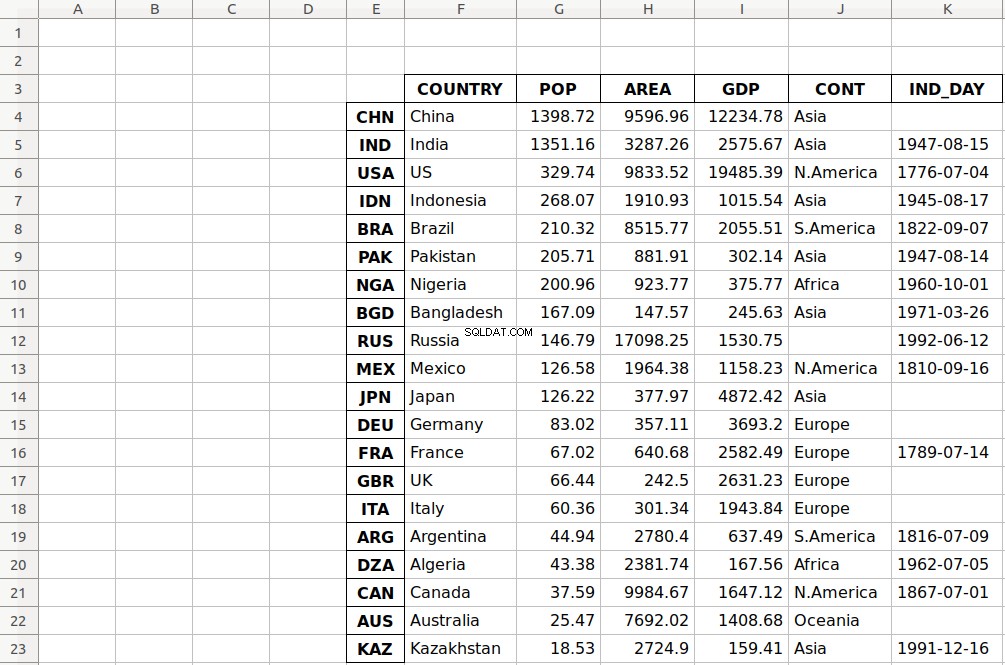
引数'data.xlsx' ターゲットファイルと、オプションでそのパスを表します。上記のステートメントは、ファイル data.xlsxを作成する必要があります 現在の作業ディレクトリにあります。そのファイルは次のようになります:
ファイルの最初の列には行のラベルが含まれ、他の列にはデータが格納されます。
Excelファイルを読む
read_excel()を使用してExcelファイルからデータを読み込むことができます :
>>> df = pd.read_excel('data.xlsx', index_col=0)
>>> df
        COUNTRY      POP      AREA       GDP       CONT     IND_DAY
CHN       China  1398.72   9596.96  12234.78       Asia         NaN
IND       India  1351.16   3287.26   2575.67       Asia  1947-08-15
USA          US   329.74   9833.52  19485.39  N.America  1776-07-04
IDN   Indonesia   268.07   1910.93   1015.54       Asia  1945-08-17
BRA      Brazil   210.32   8515.77   2055.51  S.America  1822-09-07
PAK    Pakistan   205.71    881.91    302.14       Asia  1947-08-14
NGA     Nigeria   200.96    923.77    375.77     Africa  1960-10-01
BGD  Bangladesh   167.09    147.57    245.63       Asia  1971-03-26
RUS      Russia   146.79  17098.25   1530.75        NaN  1992-06-12
MEX      Mexico   126.58   1964.38   1158.23  N.America  1810-09-16
JPN       Japan   126.22    377.97   4872.42       Asia         NaN
DEU     Germany    83.02    357.11   3693.20     Europe         NaN
FRA      France    67.02    640.68   2582.49     Europe  1789-07-14
GBR          UK    66.44    242.50   2631.23     Europe         NaN
ITA       Italy    60.36    301.34   1943.84     Europe         NaN
ARG   Argentina    44.94   2780.40    637.49  S.America  1816-07-09
DZA     Algeria    43.38   2381.74    167.56     Africa  1962-07-05
CAN      Canada    37.59   9984.67   1647.12  N.America  1867-07-01
AUS   Australia    25.47   7692.02   1408.68    Oceania         NaN
KAZ  Kazakhstan    18.53   2724.90    159.41       Asia  1991-12-16
read_excel() 新しいDataFrameを返します data.xlsxの値が含まれています 。 read_excel()を使用することもできます OpenDocumentスプレッドシート、または .odsを使用 ファイル。
このチュートリアルの後半で、Excelファイルの操作について詳しく学習します。パンダを使用してPythonで大きなExcelファイルを読み取ることも確認できます。
PandasIOAPIについて
パンダIOツール Seriesのコンテンツを保存できるAPIです およびDataFrame クリップボードへのオブジェクト、オブジェクト、またはさまざまなタイプのファイル。また、クリップボード、オブジェクト、またはファイルからデータをロードすることもできます。
ファイルの書き込み
シリーズ およびDataFrame オブジェクトには、クリップボードまたはファイルへのデータとラベルの書き込みを可能にするメソッドがあります。それらはパターン.to_ で名前が付けられています 、ここで ターゲットファイルのタイプです。
.to_csv()について学習しました および.to_excel() 、ただし、次のようなものがあります:
-
.to_json() -
.to_html() -
.to_sql() -
.to_pickle()
書き込むことができるファイルの種類はまだまだあるので、このリストは完全ではありません。
注: 同様の方法を見つけるには、 Series に関連するシリアル化、IO、および変換に関する公式ドキュメントを確認してください。 およびDataFrame オブジェクト。
これらのメソッドには、データとラベルを保存したターゲットファイルのパスを指定するパラメーターがあります。これは、必須の場合とオプションの場合があります。このオプションが使用可能であり、それを省略することを選択した場合、メソッドは DataFrame の内容を含むオブジェクト(文字列や反復可能オブジェクトなど)を返します。 インスタンス。
オプションのパラメータcompression データとラベルを使用してファイルを圧縮する方法を決定します。これについては後で詳しく説明します。他にもいくつかのパラメータがありますが、それらは主に1つまたは複数のメソッドに固有です。ここでは詳しく説明しません。
ファイルの読み取り
ファイルの内容を読み取るためのPandas関数は、パターン .read_ を使用して名前が付けられます。 、ここで 読み取るファイルのタイプを示します。パンダのread_csv()はすでにご覧になっています およびread_excel() 関数。他にもいくつかあります:
-
read_json() -
read_html() -
read_sql() -
read_pickle()
これらの関数には、ターゲットファイルのパスを指定するパラメーターがあります。これは、ローカルマシンまたはURLのいずれかでパスを表す任意の有効な文字列にすることができます。ファイルの種類によっては、他のオブジェクトも使用できます。
オプションのパラメータcompression 圧縮ファイルに使用する解凍のタイプを決定します。これについては、このチュートリアルの後半で学習します。他のパラメータもありますが、それらは1つまたは複数の関数に固有です。ここでは詳しく説明しません。
さまざまなファイルタイプの操作
Pandasライブラリは、データをファイルに保存したり、ファイルからデータをロードしたりするための幅広い可能性を提供します。このセクションでは、CSVファイルとExcelファイルの操作について詳しく学習します。また、JSON、ウェブページ、データベース、Pythonピクルスファイルなど、他の種類のファイルの使用方法についても説明します。
CSVファイル
CSVファイルの読み取りと書き込みの方法はすでに学習しました。それでは、詳細をもう少し深く掘り下げてみましょう。 .to_csv()を使用する場合 DataFrameを保存するには 、パラメータ path_or_bufの引数を指定できます ターゲットファイルのパス、名前、および拡張子を指定します。
path_or_buf 最初の引数は.to_csv() 取得します。これは、ファイル名とその拡張子を含む有効なファイルパスを表す任意の文字列にすることができます。これは前の例で見ました。ただし、 path_or_bufを省略した場合 、次に .to_csv() ファイルは作成されません。代わりに、対応する文字列を返します:
>>> df = pd.DataFrame(data=data).T
>>> s = df.to_csv()
>>> print(s)
,COUNTRY,POP,AREA,GDP,CONT,IND_DAY
CHN,China,1398.72,9596.96,12234.78,Asia,
IND,India,1351.16,3287.26,2575.67,Asia,1947-08-15
USA,US,329.74,9833.52,19485.39,N.America,1776-07-04
IDN,Indonesia,268.07,1910.93,1015.54,Asia,1945-08-17
BRA,Brazil,210.32,8515.77,2055.51,S.America,1822-09-07
PAK,Pakistan,205.71,881.91,302.14,Asia,1947-08-14
NGA,Nigeria,200.96,923.77,375.77,Africa,1960-10-01
BGD,Bangladesh,167.09,147.57,245.63,Asia,1971-03-26
RUS,Russia,146.79,17098.25,1530.75,,1992-06-12
MEX,Mexico,126.58,1964.38,1158.23,N.America,1810-09-16
JPN,Japan,126.22,377.97,4872.42,Asia,
DEU,Germany,83.02,357.11,3693.2,Europe,
FRA,France,67.02,640.68,2582.49,Europe,1789-07-14
GBR,UK,66.44,242.5,2631.23,Europe,
ITA,Italy,60.36,301.34,1943.84,Europe,
ARG,Argentina,44.94,2780.4,637.49,S.America,1816-07-09
DZA,Algeria,43.38,2381.74,167.56,Africa,1962-07-05
CAN,Canada,37.59,9984.67,1647.12,N.America,1867-07-01
AUS,Australia,25.47,7692.02,1408.68,Oceania,
KAZ,Kazakhstan,18.53,2724.9,159.41,Asia,1991-12-16
これで、文字列 sができました。 CSVファイルの代わりに。 不足している値もあります DataFrameで 物体。たとえば、ロシア大陸といくつかの国(中国、日本など)の独立日は利用できません。データサイエンスと機械学習では、欠落している値を慎重に処理する必要があります。パンダはここで優れています!デフォルトでは、PandasはNaN値を使用して欠落している値を置き換えます。
注: nan 「数値ではない」を表す、はPythonの特定の浮動小数点値です。
nanを取得できます 次の関数のいずれかを使用した値:
-
float('nan') -
math.nan -
numpy.nan
dfでロシアに対応する大陸 nanです :
>>> df.loc['RUS', 'CONT']
nan
この例では、 .loc []を使用しています 指定した行名と列名のデータを取得します。
DataFrameを保存するとき CSVファイルに、空の文字列('' )は欠落データを表します。これは、ファイル data.csvの両方で確認できます。 文字列s 。この動作を変更する場合は、オプションのパラメーター na_repを使用してください。 :
>>> df.to_csv('new-data.csv', na_rep='(missing)')
このコードは、ファイル new-data.csvを生成します 欠落している値は空の文字列ではなくなりました。以下のコードブロックを展開して、このファイルがどのように表示されるかを確認できます。
,COUNTRY,POP,AREA,GDP,CONT,IND_DAY
CHN,China,1398.72,9596.96,12234.78,Asia,(missing)
IND,India,1351.16,3287.26,2575.67,Asia,1947-08-15
USA,US,329.74,9833.52,19485.39,N.America,1776-07-04
IDN,Indonesia,268.07,1910.93,1015.54,Asia,1945-08-17
BRA,Brazil,210.32,8515.77,2055.51,S.America,1822-09-07
PAK,Pakistan,205.71,881.91,302.14,Asia,1947-08-14
NGA,Nigeria,200.96,923.77,375.77,Africa,1960-10-01
BGD,Bangladesh,167.09,147.57,245.63,Asia,1971-03-26
RUS,Russia,146.79,17098.25,1530.75,(missing),1992-06-12
MEX,Mexico,126.58,1964.38,1158.23,N.America,1810-09-16
JPN,Japan,126.22,377.97,4872.42,Asia,(missing)
DEU,Germany,83.02,357.11,3693.2,Europe,(missing)
FRA,France,67.02,640.68,2582.49,Europe,1789-07-14
GBR,UK,66.44,242.5,2631.23,Europe,(missing)
ITA,Italy,60.36,301.34,1943.84,Europe,(missing)
ARG,Argentina,44.94,2780.4,637.49,S.America,1816-07-09
DZA,Algeria,43.38,2381.74,167.56,Africa,1962-07-05
CAN,Canada,37.59,9984.67,1647.12,N.America,1867-07-01
AUS,Australia,25.47,7692.02,1408.68,Oceania,(missing)
KAZ,Kazakhstan,18.53,2724.9,159.41,Asia,1991-12-16
Now, the string '(missing)' in the file corresponds to the nan values from df 。
When Pandas reads files, it considers the empty string ('' ) and a few others as missing values by default:
'nan''-nan''NA''N/A''NaN''null'
If you don’t want this behavior, then you can pass keep_default_na=False to the Pandas read_csv() function. To specify other labels for missing values, use the parameter na_values :
>>> pd.read_csv('new-data.csv', index_col=0, na_values='(missing)')
        COUNTRY      POP      AREA       GDP       CONT     IND_DAY
CHN       China  1398.72   9596.96  12234.78       Asia         NaN
IND       India  1351.16   3287.26   2575.67       Asia  1947-08-15
USA          US   329.74   9833.52  19485.39  N.America  1776-07-04
IDN   Indonesia   268.07   1910.93   1015.54       Asia  1945-08-17
BRA      Brazil   210.32   8515.77   2055.51  S.America  1822-09-07
PAK    Pakistan   205.71    881.91    302.14       Asia  1947-08-14
NGA     Nigeria   200.96    923.77    375.77     Africa  1960-10-01
BGD  Bangladesh   167.09    147.57    245.63       Asia  1971-03-26
RUS      Russia   146.79  17098.25   1530.75        NaN  1992-06-12
MEX      Mexico   126.58   1964.38   1158.23  N.America  1810-09-16
JPN       Japan   126.22    377.97   4872.42       Asia         NaN
DEU     Germany    83.02    357.11   3693.20     Europe         NaN
FRA      France    67.02    640.68   2582.49     Europe  1789-07-14
GBR          UK    66.44    242.50   2631.23     Europe         NaN
ITA       Italy    60.36    301.34   1943.84     Europe         NaN
ARG   Argentina    44.94   2780.40    637.49  S.America  1816-07-09
DZA     Algeria    43.38   2381.74    167.56     Africa  1962-07-05
CAN      Canada    37.59   9984.67   1647.12  N.America  1867-07-01
AUS   Australia    25.47   7692.02   1408.68    Oceania         NaN
KAZ  Kazakhstan    18.53   2724.90    159.41       Asia  1991-12-16
Here, you’ve marked the string '(missing)' as a new missing data label, and Pandas replaced it with nan when it read the file.
When you load data from a file, Pandas assigns the data types to the values of each column by default. You can check these types with .dtypes :
>>> df = pd.read_csv('data.csv', index_col=0)
>>> df.dtypes
COUNTRY     object
POP        float64
AREA       float64
GDP        float64
CONT        object
IND_DAY     object
dtype: object
The columns with strings and dates ('COUNTRY' , 'CONT' , and 'IND_DAY' ) have the data type object 。 Meanwhile, the numeric columns contain 64-bit floating-point numbers (float64 。
You can use the parameter dtype to specify the desired data types and parse_dates to force use of datetimes:
>>> dtypes = {'POP': 'float32', 'AREA': 'float32', 'GDP': 'float32'}
>>> df = pd.read_csv('data.csv', index_col=0, dtype=dtypes,
...                  parse_dates=['IND_DAY'])
>>> df.dtypes
COUNTRY            object
POP               float32
AREA              float32
GDP               float32
CONT               object
IND_DAY    datetime64[ns]
dtype: object
>>> df['IND_DAY']
CHN          NaT
IND   1947-08-15
USA   1776-07-04
IDN   1945-08-17
BRA   1822-09-07
PAK   1947-08-14
NGA   1960-10-01
BGD   1971-03-26
RUS   1992-06-12
MEX   1810-09-16
JPN          NaT
DEU          NaT
FRA   1789-07-14
GBR          NaT
ITA          NaT
ARG   1816-07-09
DZA   1962-07-05
CAN   1867-07-01
AUS          NaT
KAZ   1991-12-16
Name: IND_DAY, dtype: datetime64[ns]
Now, you have 32-bit floating-point numbers (float32 ) as specified with dtype 。 These differ slightly from the original 64-bit numbers because of smaller precision 。 The values in the last column are considered as dates and have the data type datetime64 。 That’s why the NaN values in this column are replaced with NaT 。
Now that you have real dates, you can save them in the format you like:
>>>>>> df = pd.read_csv('data.csv', index_col=0, parse_dates=['IND_DAY'])
>>> df.to_csv('formatted-data.csv', date_format='%B %d, %Y')
Here, you’ve specified the parameter date_format to be '%B %d, %Y' 。 You can expand the code block below to see the resulting file:
,COUNTRY,POP,AREA,GDP,CONT,IND_DAY
CHN,China,1398.72,9596.96,12234.78,Asia,
IND,India,1351.16,3287.26,2575.67,Asia,"August 15, 1947"
USA,US,329.74,9833.52,19485.39,N.America,"July 04, 1776"
IDN,Indonesia,268.07,1910.93,1015.54,Asia,"August 17, 1945"
BRA,Brazil,210.32,8515.77,2055.51,S.America,"September 07, 1822"
PAK,Pakistan,205.71,881.91,302.14,Asia,"August 14, 1947"
NGA,Nigeria,200.96,923.77,375.77,Africa,"October 01, 1960"
BGD,Bangladesh,167.09,147.57,245.63,Asia,"March 26, 1971"
RUS,Russia,146.79,17098.25,1530.75,,"June 12, 1992"
MEX,Mexico,126.58,1964.38,1158.23,N.America,"September 16, 1810"
JPN,Japan,126.22,377.97,4872.42,Asia,
DEU,Germany,83.02,357.11,3693.2,Europe,
FRA,France,67.02,640.68,2582.49,Europe,"July 14, 1789"
GBR,UK,66.44,242.5,2631.23,Europe,
ITA,Italy,60.36,301.34,1943.84,Europe,
ARG,Argentina,44.94,2780.4,637.49,S.America,"July 09, 1816"
DZA,Algeria,43.38,2381.74,167.56,Africa,"July 05, 1962"
CAN,Canada,37.59,9984.67,1647.12,N.America,"July 01, 1867"
AUS,Australia,25.47,7692.02,1408.68,Oceania,
KAZ,Kazakhstan,18.53,2724.9,159.41,Asia,"December 16, 1991"
The format of the dates is different now. The format '%B %d, %Y' means the date will first display the full name of the month, then the day followed by a comma, and finally the full year.
There are several other optional parameters that you can use with .to_csv() :
sepdenotes a values separator.decimalindicates a decimal separator.encodingsets the file encoding.headerspecifies whether you want to write column labels in the file.
Here’s how you would pass arguments for sep and header :
>>> s = df.to_csv(sep=';', header=False)
>>> print(s)
CHN;China;1398.72;9596.96;12234.78;Asia;
IND;India;1351.16;3287.26;2575.67;Asia;1947-08-15
USA;US;329.74;9833.52;19485.39;N.America;1776-07-04
IDN;Indonesia;268.07;1910.93;1015.54;Asia;1945-08-17
BRA;Brazil;210.32;8515.77;2055.51;S.America;1822-09-07
PAK;Pakistan;205.71;881.91;302.14;Asia;1947-08-14
NGA;Nigeria;200.96;923.77;375.77;Africa;1960-10-01
BGD;Bangladesh;167.09;147.57;245.63;Asia;1971-03-26
RUS;Russia;146.79;17098.25;1530.75;;1992-06-12
MEX;Mexico;126.58;1964.38;1158.23;N.America;1810-09-16
JPN;Japan;126.22;377.97;4872.42;Asia;
DEU;Germany;83.02;357.11;3693.2;Europe;
FRA;France;67.02;640.68;2582.49;Europe;1789-07-14
GBR;UK;66.44;242.5;2631.23;Europe;
ITA;Italy;60.36;301.34;1943.84;Europe;
ARG;Argentina;44.94;2780.4;637.49;S.America;1816-07-09
DZA;Algeria;43.38;2381.74;167.56;Africa;1962-07-05
CAN;Canada;37.59;9984.67;1647.12;N.America;1867-07-01
AUS;Australia;25.47;7692.02;1408.68;Oceania;
KAZ;Kazakhstan;18.53;2724.9;159.41;Asia;1991-12-16
The data is separated with a semicolon (';' ) because you’ve specified sep=';' 。 Also, since you passed header=False , you see your data without the header row of column names.
The Pandas read_csv() function has many additional options for managing missing data, working with dates and times, quoting, encoding, handling errors, and more. For instance, if you have a file with one data column and want to get a Series object instead of a DataFrame , then you can pass squeeze=True to read_csv() 。 You’ll learn later on about data compression and decompression, as well as how to skip rows and columns.
JSON Files
JSON stands for JavaScript object notation. JSON files are plaintext files used for data interchange, and humans can read them easily. They follow the ISO/IEC 21778:2017 and ECMA-404 standards and use the .json extension. Python and Pandas work well with JSON files, as Python’s json library offers built-in support for them.
You can save the data from your DataFrame to a JSON file with .to_json() 。 Start by creating a DataFrame object again. Use the dictionary data that holds the data about countries and then apply .to_json() :
>>> df = pd.DataFrame(data=data).T
>>> df.to_json('data-columns.json')
This code produces the file data-columns.json 。 You can expand the code block below to see how this file should look:
{"COUNTRY":{"CHN":"China","IND":"India","USA":"US","IDN":"Indonesia","BRA":"Brazil","PAK":"Pakistan","NGA":"Nigeria","BGD":"Bangladesh","RUS":"Russia","MEX":"Mexico","JPN":"Japan","DEU":"Germany","FRA":"France","GBR":"UK","ITA":"Italy","ARG":"Argentina","DZA":"Algeria","CAN":"Canada","AUS":"Australia","KAZ":"Kazakhstan"},"POP":{"CHN":1398.72,"IND":1351.16,"USA":329.74,"IDN":268.07,"BRA":210.32,"PAK":205.71,"NGA":200.96,"BGD":167.09,"RUS":146.79,"MEX":126.58,"JPN":126.22,"DEU":83.02,"FRA":67.02,"GBR":66.44,"ITA":60.36,"ARG":44.94,"DZA":43.38,"CAN":37.59,"AUS":25.47,"KAZ":18.53},"AREA":{"CHN":9596.96,"IND":3287.26,"USA":9833.52,"IDN":1910.93,"BRA":8515.77,"PAK":881.91,"NGA":923.77,"BGD":147.57,"RUS":17098.25,"MEX":1964.38,"JPN":377.97,"DEU":357.11,"FRA":640.68,"GBR":242.5,"ITA":301.34,"ARG":2780.4,"DZA":2381.74,"CAN":9984.67,"AUS":7692.02,"KAZ":2724.9},"GDP":{"CHN":12234.78,"IND":2575.67,"USA":19485.39,"IDN":1015.54,"BRA":2055.51,"PAK":302.14,"NGA":375.77,"BGD":245.63,"RUS":1530.75,"MEX":1158.23,"JPN":4872.42,"DEU":3693.2,"FRA":2582.49,"GBR":2631.23,"ITA":1943.84,"ARG":637.49,"DZA":167.56,"CAN":1647.12,"AUS":1408.68,"KAZ":159.41},"CONT":{"CHN":"Asia","IND":"Asia","USA":"N.America","IDN":"Asia","BRA":"S.America","PAK":"Asia","NGA":"Africa","BGD":"Asia","RUS":null,"MEX":"N.America","JPN":"Asia","DEU":"Europe","FRA":"Europe","GBR":"Europe","ITA":"Europe","ARG":"S.America","DZA":"Africa","CAN":"N.America","AUS":"Oceania","KAZ":"Asia"},"IND_DAY":{"CHN":null,"IND":"1947-08-15","USA":"1776-07-04","IDN":"1945-08-17","BRA":"1822-09-07","PAK":"1947-08-14","NGA":"1960-10-01","BGD":"1971-03-26","RUS":"1992-06-12","MEX":"1810-09-16","JPN":null,"DEU":null,"FRA":"1789-07-14","GBR":null,"ITA":null,"ARG":"1816-07-09","DZA":"1962-07-05","CAN":"1867-07-01","AUS":null,"KAZ":"1991-12-16"}}
data-columns.json has one large dictionary with the column labels as keys and the corresponding inner dictionaries as values.
You can get a different file structure if you pass an argument for the optional parameter orient :
>>> df.to_json('data-index.json', orient='index')
The orient parameter defaults to 'columns' 。 Here, you’ve set it to index 。
You should get a new file data-index.json 。 You can expand the code block below to see the changes:
{"CHN":{"COUNTRY":"China","POP":1398.72,"AREA":9596.96,"GDP":12234.78,"CONT":"Asia","IND_DAY":null},"IND":{"COUNTRY":"India","POP":1351.16,"AREA":3287.26,"GDP":2575.67,"CONT":"Asia","IND_DAY":"1947-08-15"},"USA":{"COUNTRY":"US","POP":329.74,"AREA":9833.52,"GDP":19485.39,"CONT":"N.America","IND_DAY":"1776-07-04"},"IDN":{"COUNTRY":"Indonesia","POP":268.07,"AREA":1910.93,"GDP":1015.54,"CONT":"Asia","IND_DAY":"1945-08-17"},"BRA":{"COUNTRY":"Brazil","POP":210.32,"AREA":8515.77,"GDP":2055.51,"CONT":"S.America","IND_DAY":"1822-09-07"},"PAK":{"COUNTRY":"Pakistan","POP":205.71,"AREA":881.91,"GDP":302.14,"CONT":"Asia","IND_DAY":"1947-08-14"},"NGA":{"COUNTRY":"Nigeria","POP":200.96,"AREA":923.77,"GDP":375.77,"CONT":"Africa","IND_DAY":"1960-10-01"},"BGD":{"COUNTRY":"Bangladesh","POP":167.09,"AREA":147.57,"GDP":245.63,"CONT":"Asia","IND_DAY":"1971-03-26"},"RUS":{"COUNTRY":"Russia","POP":146.79,"AREA":17098.25,"GDP":1530.75,"CONT":null,"IND_DAY":"1992-06-12"},"MEX":{"COUNTRY":"Mexico","POP":126.58,"AREA":1964.38,"GDP":1158.23,"CONT":"N.America","IND_DAY":"1810-09-16"},"JPN":{"COUNTRY":"Japan","POP":126.22,"AREA":377.97,"GDP":4872.42,"CONT":"Asia","IND_DAY":null},"DEU":{"COUNTRY":"Germany","POP":83.02,"AREA":357.11,"GDP":3693.2,"CONT":"Europe","IND_DAY":null},"FRA":{"COUNTRY":"France","POP":67.02,"AREA":640.68,"GDP":2582.49,"CONT":"Europe","IND_DAY":"1789-07-14"},"GBR":{"COUNTRY":"UK","POP":66.44,"AREA":242.5,"GDP":2631.23,"CONT":"Europe","IND_DAY":null},"ITA":{"COUNTRY":"Italy","POP":60.36,"AREA":301.34,"GDP":1943.84,"CONT":"Europe","IND_DAY":null},"ARG":{"COUNTRY":"Argentina","POP":44.94,"AREA":2780.4,"GDP":637.49,"CONT":"S.America","IND_DAY":"1816-07-09"},"DZA":{"COUNTRY":"Algeria","POP":43.38,"AREA":2381.74,"GDP":167.56,"CONT":"Africa","IND_DAY":"1962-07-05"},"CAN":{"COUNTRY":"Canada","POP":37.59,"AREA":9984.67,"GDP":1647.12,"CONT":"N.America","IND_DAY":"1867-07-01"},"AUS":{"COUNTRY":"Australia","POP":25.47,"AREA":7692.02,"GDP":1408.68,"CONT":"Oceania","IND_DAY":null},"KAZ":{"COUNTRY":"Kazakhstan","POP":18.53,"AREA":2724.9,"GDP":159.41,"CONT":"Asia","IND_DAY":"1991-12-16"}}
data-index.json also has one large dictionary, but this time the row labels are the keys, and the inner dictionaries are the values.
There are few more options for orient 。 One of them is 'records' :
>>> df.to_json('data-records.json', orient='records')
This code should yield the file data-records.json 。 You can expand the code block below to see the content:
[{"COUNTRY":"China","POP":1398.72,"AREA":9596.96,"GDP":12234.78,"CONT":"Asia","IND_DAY":null},{"COUNTRY":"India","POP":1351.16,"AREA":3287.26,"GDP":2575.67,"CONT":"Asia","IND_DAY":"1947-08-15"},{"COUNTRY":"US","POP":329.74,"AREA":9833.52,"GDP":19485.39,"CONT":"N.America","IND_DAY":"1776-07-04"},{"COUNTRY":"Indonesia","POP":268.07,"AREA":1910.93,"GDP":1015.54,"CONT":"Asia","IND_DAY":"1945-08-17"},{"COUNTRY":"Brazil","POP":210.32,"AREA":8515.77,"GDP":2055.51,"CONT":"S.America","IND_DAY":"1822-09-07"},{"COUNTRY":"Pakistan","POP":205.71,"AREA":881.91,"GDP":302.14,"CONT":"Asia","IND_DAY":"1947-08-14"},{"COUNTRY":"Nigeria","POP":200.96,"AREA":923.77,"GDP":375.77,"CONT":"Africa","IND_DAY":"1960-10-01"},{"COUNTRY":"Bangladesh","POP":167.09,"AREA":147.57,"GDP":245.63,"CONT":"Asia","IND_DAY":"1971-03-26"},{"COUNTRY":"Russia","POP":146.79,"AREA":17098.25,"GDP":1530.75,"CONT":null,"IND_DAY":"1992-06-12"},{"COUNTRY":"Mexico","POP":126.58,"AREA":1964.38,"GDP":1158.23,"CONT":"N.America","IND_DAY":"1810-09-16"},{"COUNTRY":"Japan","POP":126.22,"AREA":377.97,"GDP":4872.42,"CONT":"Asia","IND_DAY":null},{"COUNTRY":"Germany","POP":83.02,"AREA":357.11,"GDP":3693.2,"CONT":"Europe","IND_DAY":null},{"COUNTRY":"France","POP":67.02,"AREA":640.68,"GDP":2582.49,"CONT":"Europe","IND_DAY":"1789-07-14"},{"COUNTRY":"UK","POP":66.44,"AREA":242.5,"GDP":2631.23,"CONT":"Europe","IND_DAY":null},{"COUNTRY":"Italy","POP":60.36,"AREA":301.34,"GDP":1943.84,"CONT":"Europe","IND_DAY":null},{"COUNTRY":"Argentina","POP":44.94,"AREA":2780.4,"GDP":637.49,"CONT":"S.America","IND_DAY":"1816-07-09"},{"COUNTRY":"Algeria","POP":43.38,"AREA":2381.74,"GDP":167.56,"CONT":"Africa","IND_DAY":"1962-07-05"},{"COUNTRY":"Canada","POP":37.59,"AREA":9984.67,"GDP":1647.12,"CONT":"N.America","IND_DAY":"1867-07-01"},{"COUNTRY":"Australia","POP":25.47,"AREA":7692.02,"GDP":1408.68,"CONT":"Oceania","IND_DAY":null},{"COUNTRY":"Kazakhstan","POP":18.53,"AREA":2724.9,"GDP":159.41,"CONT":"Asia","IND_DAY":"1991-12-16"}]
data-records.json holds a list with one dictionary for each row. The row labels are not written.
You can get another interesting file structure with orient='split' :
>>> df.to_json('data-split.json', orient='split')
The resulting file is data-split.json 。 You can expand the code block below to see how this file should look:
{"columns":["COUNTRY","POP","AREA","GDP","CONT","IND_DAY"],"index":["CHN","IND","USA","IDN","BRA","PAK","NGA","BGD","RUS","MEX","JPN","DEU","FRA","GBR","ITA","ARG","DZA","CAN","AUS","KAZ"],"data":[["China",1398.72,9596.96,12234.78,"Asia",null],["India",1351.16,3287.26,2575.67,"Asia","1947-08-15"],["US",329.74,9833.52,19485.39,"N.America","1776-07-04"],["Indonesia",268.07,1910.93,1015.54,"Asia","1945-08-17"],["Brazil",210.32,8515.77,2055.51,"S.America","1822-09-07"],["Pakistan",205.71,881.91,302.14,"Asia","1947-08-14"],["Nigeria",200.96,923.77,375.77,"Africa","1960-10-01"],["Bangladesh",167.09,147.57,245.63,"Asia","1971-03-26"],["Russia",146.79,17098.25,1530.75,null,"1992-06-12"],["Mexico",126.58,1964.38,1158.23,"N.America","1810-09-16"],["Japan",126.22,377.97,4872.42,"Asia",null],["Germany",83.02,357.11,3693.2,"Europe",null],["France",67.02,640.68,2582.49,"Europe","1789-07-14"],["UK",66.44,242.5,2631.23,"Europe",null],["Italy",60.36,301.34,1943.84,"Europe",null],["Argentina",44.94,2780.4,637.49,"S.America","1816-07-09"],["Algeria",43.38,2381.74,167.56,"Africa","1962-07-05"],["Canada",37.59,9984.67,1647.12,"N.America","1867-07-01"],["Australia",25.47,7692.02,1408.68,"Oceania",null],["Kazakhstan",18.53,2724.9,159.41,"Asia","1991-12-16"]]}
data-split.json contains one dictionary that holds the following lists:
- The names of the columns
- The labels of the rows
- The inner lists (two-dimensional sequence) that hold data values
If you don’t provide the value for the optional parameter path_or_buf that defines the file path, then .to_json() will return a JSON string instead of writing the results to a file. This behavior is consistent with .to_csv() 。
There are other optional parameters you can use. For instance, you can set index=False to forgo saving row labels. You can manipulate precision with double_precision , and dates with date_format and date_unit 。 These last two parameters are particularly important when you have time series among your data:
>>> df = pd.DataFrame(data=data).T
>>> df['IND_DAY'] = pd.to_datetime(df['IND_DAY'])
>>> df.dtypes
COUNTRY            object
POP                object
AREA               object
GDP                object
CONT               object
IND_DAY    datetime64[ns]
dtype: object

>>> df.to_json('data-time.json')
In this example, you’ve created the DataFrame from the dictionary data and used to_datetime() to convert the values in the last column to datetime64 。 You can expand the code block below to see the resulting file:
{"COUNTRY":{"CHN":"China","IND":"India","USA":"US","IDN":"Indonesia","BRA":"Brazil","PAK":"Pakistan","NGA":"Nigeria","BGD":"Bangladesh","RUS":"Russia","MEX":"Mexico","JPN":"Japan","DEU":"Germany","FRA":"France","GBR":"UK","ITA":"Italy","ARG":"Argentina","DZA":"Algeria","CAN":"Canada","AUS":"Australia","KAZ":"Kazakhstan"},"POP":{"CHN":1398.72,"IND":1351.16,"USA":329.74,"IDN":268.07,"BRA":210.32,"PAK":205.71,"NGA":200.96,"BGD":167.09,"RUS":146.79,"MEX":126.58,"JPN":126.22,"DEU":83.02,"FRA":67.02,"GBR":66.44,"ITA":60.36,"ARG":44.94,"DZA":43.38,"CAN":37.59,"AUS":25.47,"KAZ":18.53},"AREA":{"CHN":9596.96,"IND":3287.26,"USA":9833.52,"IDN":1910.93,"BRA":8515.77,"PAK":881.91,"NGA":923.77,"BGD":147.57,"RUS":17098.25,"MEX":1964.38,"JPN":377.97,"DEU":357.11,"FRA":640.68,"GBR":242.5,"ITA":301.34,"ARG":2780.4,"DZA":2381.74,"CAN":9984.67,"AUS":7692.02,"KAZ":2724.9},"GDP":{"CHN":12234.78,"IND":2575.67,"USA":19485.39,"IDN":1015.54,"BRA":2055.51,"PAK":302.14,"NGA":375.77,"BGD":245.63,"RUS":1530.75,"MEX":1158.23,"JPN":4872.42,"DEU":3693.2,"FRA":2582.49,"GBR":2631.23,"ITA":1943.84,"ARG":637.49,"DZA":167.56,"CAN":1647.12,"AUS":1408.68,"KAZ":159.41},"CONT":{"CHN":"Asia","IND":"Asia","USA":"N.America","IDN":"Asia","BRA":"S.America","PAK":"Asia","NGA":"Africa","BGD":"Asia","RUS":null,"MEX":"N.America","JPN":"Asia","DEU":"Europe","FRA":"Europe","GBR":"Europe","ITA":"Europe","ARG":"S.America","DZA":"Africa","CAN":"N.America","AUS":"Oceania","KAZ":"Asia"},"IND_DAY":{"CHN":null,"IND":-706320000000,"USA":-6106060800000,"IDN":-769219200000,"BRA":-4648924800000,"PAK":-706406400000,"NGA":-291945600000,"BGD":38793600000,"RUS":708307200000,"MEX":-5026838400000,"JPN":null,"DEU":null,"FRA":-5694969600000,"GBR":null,"ITA":null,"ARG":-4843411200000,"DZA":-236476800000,"CAN":-3234729600000,"AUS":null,"KAZ":692841600000}}
In this file, you have large integers instead of dates for the independence days. That’s because the default value of the optional parameter date_format is 'epoch' whenever orient isn’t 'table' 。 This default behavior expresses dates as an epoch in milliseconds relative to midnight on January 1, 1970.
However, if you pass date_format='iso' , then you’ll get the dates in the ISO 8601 format. In addition, date_unit decides the units of time:
>>> df = pd.DataFrame(data=data).T
>>> df['IND_DAY'] = pd.to_datetime(df['IND_DAY'])
>>> df.to_json('new-data-time.json', date_format='iso', date_unit='s')
This code produces the following JSON file:
{"COUNTRY":{"CHN":"China","IND":"India","USA":"US","IDN":"Indonesia","BRA":"Brazil","PAK":"Pakistan","NGA":"Nigeria","BGD":"Bangladesh","RUS":"Russia","MEX":"Mexico","JPN":"Japan","DEU":"Germany","FRA":"France","GBR":"UK","ITA":"Italy","ARG":"Argentina","DZA":"Algeria","CAN":"Canada","AUS":"Australia","KAZ":"Kazakhstan"},"POP":{"CHN":1398.72,"IND":1351.16,"USA":329.74,"IDN":268.07,"BRA":210.32,"PAK":205.71,"NGA":200.96,"BGD":167.09,"RUS":146.79,"MEX":126.58,"JPN":126.22,"DEU":83.02,"FRA":67.02,"GBR":66.44,"ITA":60.36,"ARG":44.94,"DZA":43.38,"CAN":37.59,"AUS":25.47,"KAZ":18.53},"AREA":{"CHN":9596.96,"IND":3287.26,"USA":9833.52,"IDN":1910.93,"BRA":8515.77,"PAK":881.91,"NGA":923.77,"BGD":147.57,"RUS":17098.25,"MEX":1964.38,"JPN":377.97,"DEU":357.11,"FRA":640.68,"GBR":242.5,"ITA":301.34,"ARG":2780.4,"DZA":2381.74,"CAN":9984.67,"AUS":7692.02,"KAZ":2724.9},"GDP":{"CHN":12234.78,"IND":2575.67,"USA":19485.39,"IDN":1015.54,"BRA":2055.51,"PAK":302.14,"NGA":375.77,"BGD":245.63,"RUS":1530.75,"MEX":1158.23,"JPN":4872.42,"DEU":3693.2,"FRA":2582.49,"GBR":2631.23,"ITA":1943.84,"ARG":637.49,"DZA":167.56,"CAN":1647.12,"AUS":1408.68,"KAZ":159.41},"CONT":{"CHN":"Asia","IND":"Asia","USA":"N.America","IDN":"Asia","BRA":"S.America","PAK":"Asia","NGA":"Africa","BGD":"Asia","RUS":null,"MEX":"N.America","JPN":"Asia","DEU":"Europe","FRA":"Europe","GBR":"Europe","ITA":"Europe","ARG":"S.America","DZA":"Africa","CAN":"N.America","AUS":"Oceania","KAZ":"Asia"},"IND_DAY":{"CHN":null,"IND":"1947-08-15T00:00:00Z","USA":"1776-07-04T00:00:00Z","IDN":"1945-08-17T00:00:00Z","BRA":"1822-09-07T00:00:00Z","PAK":"1947-08-14T00:00:00Z","NGA":"1960-10-01T00:00:00Z","BGD":"1971-03-26T00:00:00Z","RUS":"1992-06-12T00:00:00Z","MEX":"1810-09-16T00:00:00Z","JPN":null,"DEU":null,"FRA":"1789-07-14T00:00:00Z","GBR":null,"ITA":null,"ARG":"1816-07-09T00:00:00Z","DZA":"1962-07-05T00:00:00Z","CAN":"1867-07-01T00:00:00Z","AUS":null,"KAZ":"1991-12-16T00:00:00Z"}}
The dates in the resulting file are in the ISO 8601 format.
You can load the data from a JSON file with read_json() :
>>> df = pd.read_json('data-index.json', orient='index',
...                   convert_dates=['IND_DAY'])
The parameter convert_dates has a similar purpose as parse_dates when you use it to read CSV files. The optional parameter orient is very important because it specifies how Pandas understands the structure of the file.
There are other optional parameters you can use as well:
- Set the encoding with
encoding. - Manipulate dates with
convert_datesandkeep_default_dates. - Impact precision with
dtypeandprecise_float. - Decode numeric data directly to NumPy arrays with
numpy=True.
Note that you might lose the order of rows and columns when using the JSON format to store your data.
HTML Files
An HTML is a plaintext file that uses hypertext markup language to help browsers render web pages. The extensions for HTML files are .html and .htm 。 You’ll need to install an HTML parser library like lxml or html5lib to be able to work with HTML files:
$pip install lxml html5lib
You can also use Conda to install the same packages:
$ conda install lxml html5lib
Once you have these libraries, you can save the contents of your DataFrame as an HTML file with .to_html() :
df = pd.DataFrame(data=data).T
df.to_html('data.html')
This code generates a file data.html 。 You can expand the code block below to see how this file should look:
<table border="1" class="dataframe">
  <thead>
    <tr style="text-align: right;">
      <th></th>
      <th>COUNTRY</th>
      <th>POP</th>
      <th>AREA</th>
      <th>GDP</th>
      <th>CONT</th>
      <th>IND_DAY</th>
    </tr>
  </thead>
  <tbody>
    <tr>
      <th>CHN</th>
      <td>China</td>
      <td>1398.72</td>
      <td>9596.96</td>
      <td>12234.8</td>
      <td>Asia</td>
      <td>NaN</td>
    </tr>
    <tr>
      <th>IND</th>
      <td>India</td>
      <td>1351.16</td>
      <td>3287.26</td>
      <td>2575.67</td>
      <td>Asia</td>
      <td>1947-08-15</td>
    </tr>
    <tr>
      <th>USA</th>
      <td>US</td>
      <td>329.74</td>
      <td>9833.52</td>
      <td>19485.4</td>
      <td>N.America</td>
      <td>1776-07-04</td>
    </tr>
    <tr>
      <th>IDN</th>
      <td>Indonesia</td>
      <td>268.07</td>
      <td>1910.93</td>
      <td>1015.54</td>
      <td>Asia</td>
      <td>1945-08-17</td>
    </tr>
    <tr>
      <th>BRA</th>
      <td>Brazil</td>
      <td>210.32</td>
      <td>8515.77</td>
      <td>2055.51</td>
      <td>S.America</td>
      <td>1822-09-07</td>
    </tr>
    <tr>
      <th>PAK</th>
      <td>Pakistan</td>
      <td>205.71</td>
      <td>881.91</td>
      <td>302.14</td>
      <td>Asia</td>
      <td>1947-08-14</td>
    </tr>
    <tr>
      <th>NGA</th>
      <td>Nigeria</td>
      <td>200.96</td>
      <td>923.77</td>
      <td>375.77</td>
      <td>Africa</td>
      <td>1960-10-01</td>
    </tr>
    <tr>
      <th>BGD</th>
      <td>Bangladesh</td>
      <td>167.09</td>
      <td>147.57</td>
      <td>245.63</td>
      <td>Asia</td>
      <td>1971-03-26</td>
    </tr>
    <tr>
      <th>RUS</th>
      <td>Russia</td>
      <td>146.79</td>
      <td>17098.2</td>
      <td>1530.75</td>
      <td>NaN</td>
      <td>1992-06-12</td>
    </tr>
    <tr>
      <th>MEX</th>
      <td>Mexico</td>
      <td>126.58</td>
      <td>1964.38</td>
      <td>1158.23</td>
      <td>N.America</td>
      <td>1810-09-16</td>
    </tr>
    <tr>
      <th>JPN</th>
      <td>Japan</td>
      <td>126.22</td>
      <td>377.97</td>
      <td>4872.42</td>
      <td>Asia</td>
      <td>NaN</td>
    </tr>
    <tr>
      <th>DEU</th>
      <td>Germany</td>
      <td>83.02</td>
      <td>357.11</td>
      <td>3693.2</td>
      <td>Europe</td>
      <td>NaN</td>
    </tr>
    <tr>
      <th>FRA</th>
      <td>France</td>
      <td>67.02</td>
      <td>640.68</td>
      <td>2582.49</td>
      <td>Europe</td>
      <td>1789-07-14</td>
    </tr>
    <tr>
      <th>GBR</th>
      <td>UK</td>
      <td>66.44</td>
      <td>242.5</td>
      <td>2631.23</td>
      <td>Europe</td>
      <td>NaN</td>
    </tr>
    <tr>
      <th>ITA</th>
      <td>Italy</td>
      <td>60.36</td>
      <td>301.34</td>
      <td>1943.84</td>
      <td>Europe</td>
      <td>NaN</td>
    </tr>
    <tr>
      <th>ARG</th>
      <td>Argentina</td>
      <td>44.94</td>
      <td>2780.4</td>
      <td>637.49</td>
      <td>S.America</td>
      <td>1816-07-09</td>
    </tr>
    <tr>
      <th>DZA</th>
      <td>Algeria</td>
      <td>43.38</td>
      <td>2381.74</td>
      <td>167.56</td>
      <td>Africa</td>
      <td>1962-07-05</td>
    </tr>
    <tr>
      <th>CAN</th>
      <td>Canada</td>
      <td>37.59</td>
      <td>9984.67</td>
      <td>1647.12</td>
      <td>N.America</td>
      <td>1867-07-01</td>
    </tr>
    <tr>
      <th>AUS</th>
      <td>Australia</td>
      <td>25.47</td>
      <td>7692.02</td>
      <td>1408.68</td>
      <td>Oceania</td>
      <td>NaN</td>
    </tr>
    <tr>
      <th>KAZ</th>
      <td>Kazakhstan</td>
      <td>18.53</td>
      <td>2724.9</td>
      <td>159.41</td>
      <td>Asia</td>
      <td>1991-12-16</td>
    </tr>
  </tbody>
</table>
This file shows the DataFrame contents nicely. However, notice that you haven’t obtained an entire web page. You’ve just output the data that corresponds to df in the HTML format.
.to_html() won’t create a file if you don’t provide the optional parameter buf , which denotes the buffer to write to. If you leave this parameter out, then your code will return a string as it did with .to_csv() and .to_json() 。
Here are some other optional parameters:
headerdetermines whether to save the column names.indexdetermines whether to save the row labels.classesassigns cascading style sheet (CSS) classes.render_linksspecifies whether to convert URLs to HTML links.table_idassigns the CSSidto thetabletag.escapedecides whether to convert the characters<,>, and&to HTML-safe strings.
You use parameters like these to specify different aspects of the resulting files or strings.
You can create a DataFrame object from a suitable HTML file using read_html() , which will return a DataFrame instance or a list of them:
>>> df = pd.read_html('data.html', index_col=0, parse_dates=['IND_DAY'])
This is very similar to what you did when reading CSV files. You also have parameters that help you work with dates, missing values, precision, encoding, HTML parsers, and more.
Excel Files
You’ve already learned how to read and write Excel files with Pandas. However, there are a few more options worth considering. For one, when you use .to_excel() , you can specify the name of the target worksheet with the optional parameter sheet_name :
>>> df = pd.DataFrame(data=data).T
>>> df.to_excel('data.xlsx', sheet_name='COUNTRIES')
Here, you create a file data.xlsx with a worksheet called COUNTRIES that stores the data. The string 'data.xlsx' is the argument for the parameter excel_writer that defines the name of the Excel file or its path.
The optional parameters startrow and startcol both default to 0 and indicate the upper left-most cell where the data should start being written:
>>> df.to_excel('data-shifted.xlsx', sheet_name='COUNTRIES',
...             startrow=2, startcol=4)
Here, you specify that the table should start in the third row and the fifth column. You also used zero-based indexing, so the third row is denoted by 2 and the fifth column by 4 。
Now the resulting worksheet looks like this:
As you can see, the table starts in the third row 2 and the fifth column E 。
.read_excel() also has the optional parameter sheet_name that specifies which worksheets to read when loading data. It can take on one of the following values:
- The zero-based index of the worksheet
- The name of the worksheet
- The list of indices or names to read multiple sheets
- The value
Noneto read all sheets
Here’s how you would use this parameter in your code:
>>>>>> df = pd.read_excel('data.xlsx', sheet_name=0, index_col=0,
... parse_dates=['IND_DAY'])
>>> df = pd.read_excel('data.xlsx', sheet_name='COUNTRIES', index_col=0,
... parse_dates=['IND_DAY'])
Both statements above create the same DataFrame because the sheet_name parameters have the same values. In both cases, sheet_name=0 and sheet_name='COUNTRIES' refer to the same worksheet. The argument parse_dates=['IND_DAY'] tells Pandas to try to consider the values in this column as dates or times.
There are other optional parameters you can use with .read_excel() and .to_excel() to determine the Excel engine, the encoding, the way to handle missing values and infinities, the method for writing column names and row labels, and so on.
SQL Files
Pandas IO tools can also read and write databases. In this next example, you’ll write your data to a database called data.db 。 To get started, you’ll need the SQLAlchemy package. To learn more about it, you can read the official ORM tutorial. You’ll also need the database driver. Python has a built-in driver for SQLite.
You can install SQLAlchemy with pip:
$ pip install sqlalchemy
You can also install it with Conda:
$ conda install sqlalchemy
Once you have SQLAlchemy installed, import create_engine() and create a database engine:
>>> from sqlalchemy import create_engine
>>> engine = create_engine('sqlite:///data.db', echo=False)
Now that you have everything set up, the next step is to create a DataFrame object. It’s convenient to specify the data types and apply .to_sql() 。
>>> dtypes = {'POP': 'float64', 'AREA': 'float64', 'GDP': 'float64',
...           'IND_DAY': 'datetime64'}
>>> df = pd.DataFrame(data=data).T.astype(dtype=dtypes)
>>> df.dtypes
COUNTRY            object
POP               float64
AREA              float64
GDP               float64
CONT               object
IND_DAY    datetime64[ns]
dtype: object
.astype() is a very convenient method you can use to set multiple data types at once.
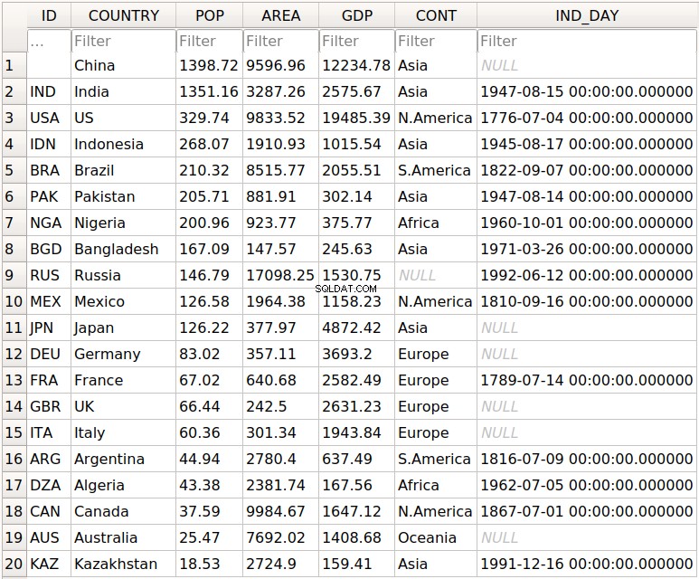
Once you’ve created your DataFrame , you can save it to the database with .to_sql() :
>>> df.to_sql('data.db', con=engine, index_label='ID')
The parameter con is used to specify the database connection or engine that you want to use. The optional parameter index_label specifies how to call the database column with the row labels. You’ll often see it take on the value ID , Id , or id 。
You should get the database data.db with a single table that looks like this:
The first column contains the row labels. To omit writing them into the database, pass index=False to .to_sql() 。 The other columns correspond to the columns of the DataFrame 。
There are a few more optional parameters. For example, you can use schema to specify the database schema and dtype to determine the types of the database columns. You can also use if_exists , which says what to do if a database with the same name and path already exists:
if_exists='fail'raises a ValueError and is the default.if_exists='replace'drops the table and inserts new values.if_exists='append'inserts new values into the table.
You can load the data from the database with read_sql() :
>>> df = pd.read_sql('data.db', con=engine, index_col='ID')
>>> df
        COUNTRY      POP      AREA       GDP       CONT    IND_DAY
ID
CHN       China  1398.72   9596.96  12234.78       Asia        NaT
IND       India  1351.16   3287.26   2575.67       Asia 1947-08-15
USA          US   329.74   9833.52  19485.39  N.America 1776-07-04
IDN   Indonesia   268.07   1910.93   1015.54       Asia 1945-08-17
BRA      Brazil   210.32   8515.77   2055.51  S.America 1822-09-07
PAK    Pakistan   205.71    881.91    302.14       Asia 1947-08-14
NGA     Nigeria   200.96    923.77    375.77     Africa 1960-10-01
BGD  Bangladesh   167.09    147.57    245.63       Asia 1971-03-26
RUS      Russia   146.79  17098.25   1530.75       None 1992-06-12
MEX      Mexico   126.58   1964.38   1158.23  N.America 1810-09-16
JPN       Japan   126.22    377.97   4872.42       Asia        NaT
DEU     Germany    83.02    357.11   3693.20     Europe        NaT
FRA      France    67.02    640.68   2582.49     Europe 1789-07-14
GBR          UK    66.44    242.50   2631.23     Europe        NaT
ITA       Italy    60.36    301.34   1943.84     Europe        NaT
ARG   Argentina    44.94   2780.40    637.49  S.America 1816-07-09
DZA     Algeria    43.38   2381.74    167.56     Africa 1962-07-05
CAN      Canada    37.59   9984.67   1647.12  N.America 1867-07-01
AUS   Australia    25.47   7692.02   1408.68    Oceania        NaT
KAZ  Kazakhstan    18.53   2724.90    159.41       Asia 1991-12-16
The parameter index_col specifies the name of the column with the row labels. Note that this inserts an extra row after the header that starts with ID 。 You can fix this behavior with the following line of code:
>>> df.index.name = None
>>> df
        COUNTRY      POP      AREA       GDP       CONT    IND_DAY
CHN       China  1398.72   9596.96  12234.78       Asia        NaT
IND       India  1351.16   3287.26   2575.67       Asia 1947-08-15
USA          US   329.74   9833.52  19485.39  N.America 1776-07-04
IDN   Indonesia   268.07   1910.93   1015.54       Asia 1945-08-17
BRA      Brazil   210.32   8515.77   2055.51  S.America 1822-09-07
PAK    Pakistan   205.71    881.91    302.14       Asia 1947-08-14
NGA     Nigeria   200.96    923.77    375.77     Africa 1960-10-01
BGD  Bangladesh   167.09    147.57    245.63       Asia 1971-03-26
RUS      Russia   146.79  17098.25   1530.75       None 1992-06-12
MEX      Mexico   126.58   1964.38   1158.23  N.America 1810-09-16
JPN       Japan   126.22    377.97   4872.42       Asia        NaT
DEU     Germany    83.02    357.11   3693.20     Europe        NaT
FRA      France    67.02    640.68   2582.49     Europe 1789-07-14
GBR          UK    66.44    242.50   2631.23     Europe        NaT
ITA       Italy    60.36    301.34   1943.84     Europe        NaT
ARG   Argentina    44.94   2780.40    637.49  S.America 1816-07-09
DZA     Algeria    43.38   2381.74    167.56     Africa 1962-07-05
CAN      Canada    37.59   9984.67   1647.12  N.America 1867-07-01
AUS   Australia    25.47   7692.02   1408.68    Oceania        NaT
KAZ  Kazakhstan    18.53   2724.90    159.41       Asia 1991-12-16
Now you have the same DataFrame object as before.
Note that the continent for Russia is now None instead of nan 。 If you want to fill the missing values with nan , then you can use .fillna() :
>>> df.fillna(value=float('nan'), inplace=True)
.fillna() replaces all missing values with whatever you pass to value 。 Here, you passed float('nan') , which says to fill all missing values with nan 。
Also note that you didn’t have to pass parse_dates=['IND_DAY'] to read_sql() 。 That’s because your database was able to detect that the last column contains dates. However, you can pass parse_dates if you’d like. You’ll get the same results.
There are other functions that you can use to read databases, like read_sql_table() and read_sql_query() 。 Feel free to try them out!
Pickle Files
Pickling is the act of converting Python objects into byte streams. Unpickling is the inverse process. Python pickle files are the binary files that keep the data and hierarchy of Python objects. They usually have the extension .pickle or .pkl 。
You can save your DataFrame in a pickle file with .to_pickle() :
>>> dtypes = {'POP': 'float64', 'AREA': 'float64', 'GDP': 'float64',
...           'IND_DAY': 'datetime64'}
>>> df = pd.DataFrame(data=data).T.astype(dtype=dtypes)
>>> df.to_pickle('data.pickle')
Like you did with databases, it can be convenient first to specify the data types. Then, you create a file data.pickle to contain your data. You could also pass an integer value to the optional parameter protocol , which specifies the protocol of the pickler.
You can get the data from a pickle file with read_pickle() :
>>> df = pd.read_pickle('data.pickle')
>>> df
        COUNTRY      POP      AREA       GDP       CONT    IND_DAY
CHN       China  1398.72   9596.96  12234.78       Asia        NaT
IND       India  1351.16   3287.26   2575.67       Asia 1947-08-15
USA          US   329.74   9833.52  19485.39  N.America 1776-07-04
IDN   Indonesia   268.07   1910.93   1015.54       Asia 1945-08-17
BRA      Brazil   210.32   8515.77   2055.51  S.America 1822-09-07
PAK    Pakistan   205.71    881.91    302.14       Asia 1947-08-14
NGA     Nigeria   200.96    923.77    375.77     Africa 1960-10-01
BGD  Bangladesh   167.09    147.57    245.63       Asia 1971-03-26
RUS      Russia   146.79  17098.25   1530.75        NaN 1992-06-12
MEX      Mexico   126.58   1964.38   1158.23  N.America 1810-09-16
JPN       Japan   126.22    377.97   4872.42       Asia        NaT
DEU     Germany    83.02    357.11   3693.20     Europe        NaT
FRA      France    67.02    640.68   2582.49     Europe 1789-07-14
GBR          UK    66.44    242.50   2631.23     Europe        NaT
ITA       Italy    60.36    301.34   1943.84     Europe        NaT
ARG   Argentina    44.94   2780.40    637.49  S.America 1816-07-09
DZA     Algeria    43.38   2381.74    167.56     Africa 1962-07-05
CAN      Canada    37.59   9984.67   1647.12  N.America 1867-07-01
AUS   Australia    25.47   7692.02   1408.68    Oceania        NaT
KAZ  Kazakhstan    18.53   2724.90    159.41       Asia 1991-12-16
read_pickle() returns the DataFrame with the stored data. You can also check the data types:
>>> df.dtypes
COUNTRY            object
POP               float64
AREA              float64
GDP               float64
CONT               object
IND_DAY    datetime64[ns]
dtype: object
These are the same ones that you specified before using .to_pickle() 。
As a word of caution, you should always beware of loading pickles from untrusted sources. This can be dangerous! When you unpickle an untrustworthy file, it could execute arbitrary code on your machine, gain remote access to your computer, or otherwise exploit your device in other ways.
Working With Big Data
If your files are too large for saving or processing, then there are several approaches you can take to reduce the required disk space:
- Compress your files
- Choose only the columns you want
- Omit the rows you don’t need
- Force the use of less precise data types
- Split the data into chunks
You’ll take a look at each of these techniques in turn.
Compress and Decompress Files
You can create an archive file like you would a regular one, with the addition of a suffix that corresponds to the desired compression type:
'.gz''.bz2''.zip''.xz'
Pandas can deduce the compression type by itself:
>>>>>> df = pd.DataFrame(data=data).T
>>> df.to_csv('data.csv.zip')
Here, you create a compressed .csv file as an archive. The size of the regular .csv file is 1048 bytes, while the compressed file only has 766 bytes.
You can open this compressed file as usual with the Pandas read_csv() function:
>>> df = pd.read_csv('data.csv.zip', index_col=0,
...                  parse_dates=['IND_DAY'])
>>> df
        COUNTRY      POP      AREA       GDP       CONT    IND_DAY
CHN       China  1398.72   9596.96  12234.78       Asia        NaT
IND       India  1351.16   3287.26   2575.67       Asia 1947-08-15
USA          US   329.74   9833.52  19485.39  N.America 1776-07-04
IDN   Indonesia   268.07   1910.93   1015.54       Asia 1945-08-17
BRA      Brazil   210.32   8515.77   2055.51  S.America 1822-09-07
PAK    Pakistan   205.71    881.91    302.14       Asia 1947-08-14
NGA     Nigeria   200.96    923.77    375.77     Africa 1960-10-01
BGD  Bangladesh   167.09    147.57    245.63       Asia 1971-03-26
RUS      Russia   146.79  17098.25   1530.75        NaN 1992-06-12
MEX      Mexico   126.58   1964.38   1158.23  N.America 1810-09-16
JPN       Japan   126.22    377.97   4872.42       Asia        NaT
DEU     Germany    83.02    357.11   3693.20     Europe        NaT
FRA      France    67.02    640.68   2582.49     Europe 1789-07-14
GBR          UK    66.44    242.50   2631.23     Europe        NaT
ITA       Italy    60.36    301.34   1943.84     Europe        NaT
ARG   Argentina    44.94   2780.40    637.49  S.America 1816-07-09
DZA     Algeria    43.38   2381.74    167.56     Africa 1962-07-05
CAN      Canada    37.59   9984.67   1647.12  N.America 1867-07-01
AUS   Australia    25.47   7692.02   1408.68    Oceania        NaT
KAZ  Kazakhstan    18.53   2724.90    159.41       Asia 1991-12-16
read_csv() decompresses the file before reading it into a DataFrame 。
You can specify the type of compression with the optional parameter compression , which can take on any of the following values:
'infer''gzip''bz2''zip''xz'None
The default value compression='infer' indicates that Pandas should deduce the compression type from the file extension.
Here’s how you would compress a pickle file:
>>>>>> df = pd.DataFrame(data=data).T
>>> df.to_pickle('data.pickle.compress', compression='gzip')
You should get the file data.pickle.compress that you can later decompress and read:
>>> df = pd.read_pickle('data.pickle.compress', compression='gzip')
df again corresponds to the DataFrame with the same data as before.
You can give the other compression methods a try, as well. If you’re using pickle files, then keep in mind that the .zip format supports reading only.
Choose Columns
The Pandas read_csv() and read_excel() functions have the optional parameter usecols that you can use to specify the columns you want to load from the file. You can pass the list of column names as the corresponding argument:
>>> df = pd.read_csv('data.csv', usecols=['COUNTRY', 'AREA'])
>>> df
       COUNTRY      AREA
0        China   9596.96
1        India   3287.26
2           US   9833.52
3    Indonesia   1910.93
4       Brazil   8515.77
5     Pakistan    881.91
6      Nigeria    923.77
7   Bangladesh    147.57
8       Russia  17098.25
9       Mexico   1964.38
10       Japan    377.97
11     Germany    357.11
12      France    640.68
13          UK    242.50
14       Italy    301.34
15   Argentina   2780.40
16     Algeria   2381.74
17      Canada   9984.67
18   Australia   7692.02
19  Kazakhstan   2724.90
Now you have a DataFrame that contains less data than before. Here, there are only the names of the countries and their areas.
Instead of the column names, you can also pass their indices:
>>>>>> df = pd.read_csv('data.csv',index_col=0, usecols=[0, 1, 3])
>>> df
COUNTRY AREA
CHN China 9596.96
IND India 3287.26
USA US 9833.52
IDN Indonesia 1910.93
BRA Brazil 8515.77
PAK Pakistan 881.91
NGA Nigeria 923.77
BGD Bangladesh 147.57
RUS Russia 17098.25
MEX Mexico 1964.38
JPN Japan 377.97
DEU Germany 357.11
FRA France 640.68
GBR UK 242.50
ITA Italy 301.34
ARG Argentina 2780.40
DZA Algeria 2381.74
CAN Canada 9984.67
AUS Australia 7692.02
KAZ Kazakhstan 2724.90
Expand the code block below to compare these results with the file 'data.csv' :
,COUNTRY,POP,AREA,GDP,CONT,IND_DAY
CHN,China,1398.72,9596.96,12234.78,Asia,
IND,India,1351.16,3287.26,2575.67,Asia,1947-08-15
USA,US,329.74,9833.52,19485.39,N.America,1776-07-04
IDN,Indonesia,268.07,1910.93,1015.54,Asia,1945-08-17
BRA,Brazil,210.32,8515.77,2055.51,S.America,1822-09-07
PAK,Pakistan,205.71,881.91,302.14,Asia,1947-08-14
NGA,Nigeria,200.96,923.77,375.77,Africa,1960-10-01
BGD,Bangladesh,167.09,147.57,245.63,Asia,1971-03-26
RUS,Russia,146.79,17098.25,1530.75,,1992-06-12
MEX,Mexico,126.58,1964.38,1158.23,N.America,1810-09-16
JPN,Japan,126.22,377.97,4872.42,Asia,
DEU,Germany,83.02,357.11,3693.2,Europe,
FRA,France,67.02,640.68,2582.49,Europe,1789-07-14
GBR,UK,66.44,242.5,2631.23,Europe,
ITA,Italy,60.36,301.34,1943.84,Europe,
ARG,Argentina,44.94,2780.4,637.49,S.America,1816-07-09
DZA,Algeria,43.38,2381.74,167.56,Africa,1962-07-05
CAN,Canada,37.59,9984.67,1647.12,N.America,1867-07-01
AUS,Australia,25.47,7692.02,1408.68,Oceania,
KAZ,Kazakhstan,18.53,2724.9,159.41,Asia,1991-12-16
You can see the following columns:
- The column at index
0contains the row labels. - The column at index
1contains the country names. - The column at index
3contains the areas.
Simlarly, read_sql() has the optional parameter columns that takes a list of column names to read:
>>> df = pd.read_sql('data.db', con=engine, index_col='ID',
...                  columns=['COUNTRY', 'AREA'])
>>> df.index.name = None
>>> df
        COUNTRY      AREA
CHN       China   9596.96
IND       India   3287.26
USA          US   9833.52
IDN   Indonesia   1910.93
BRA      Brazil   8515.77
PAK    Pakistan    881.91
NGA     Nigeria    923.77
BGD  Bangladesh    147.57
RUS      Russia  17098.25
MEX      Mexico   1964.38
JPN       Japan    377.97
DEU     Germany    357.11
FRA      France    640.68
GBR          UK    242.50
ITA       Italy    301.34
ARG   Argentina   2780.40
DZA     Algeria   2381.74
CAN      Canada   9984.67
AUS   Australia   7692.02
KAZ  Kazakhstan   2724.90
Again, the DataFrame only contains the columns with the names of the countries and areas. If columns is None or omitted, then all of the columns will be read, as you saw before. The default behavior is columns=None 。
Omit Rows
When you test an algorithm for data processing or machine learning, you often don’t need the entire dataset. It’s convenient to load only a subset of the data to speed up the process. The Pandas read_csv() and read_excel() functions have some optional parameters that allow you to select which rows you want to load:
skiprows: either the number of rows to skip at the beginning of the file if it’s an integer, or the zero-based indices of the rows to skip if it’s a list-like objectskipfooter: the number of rows to skip at the end of the filenrows: the number of rows to read
Here’s how you would skip rows with odd zero-based indices, keeping the even ones:
>>>>>> df = pd.read_csv('data.csv', index_col=0, skiprows=range(1, 20, 2))
>>> df
COUNTRY POP AREA GDP CONT IND_DAY
IND India 1351.16 3287.26 2575.67 Asia 1947-08-15
IDN Indonesia 268.07 1910.93 1015.54 Asia 1945-08-17
PAK Pakistan 205.71 881.91 302.14 Asia 1947-08-14
BGD Bangladesh 167.09 147.57 245.63 Asia 1971-03-26
MEX Mexico 126.58 1964.38 1158.23 N.America 1810-09-16
DEU Germany 83.02 357.11 3693.20 Europe NaN
GBR UK 66.44 242.50 2631.23 Europe NaN
ARG Argentina 44.94 2780.40 637.49 S.America 1816-07-09
CAN Canada 37.59 9984.67 1647.12 N.America 1867-07-01
KAZ Kazakhstan 18.53 2724.90 159.41 Asia 1991-12-16
In this example, skiprows is range(1, 20, 2) and corresponds to the values 1 , 3 , …, 19 。 The instances of the Python built-in class range behave like sequences. The first row of the file data.csv is the header row. It has the index 0 , so Pandas loads it in. The second row with index 1 corresponds to the label CHN , and Pandas skips it. The third row with the index 2 and label IND is loaded, and so on.
If you want to choose rows randomly, then skiprows can be a list or NumPy array with pseudo-random numbers, obtained either with pure Python or with NumPy.
Force Less Precise Data Types
If you’re okay with less precise data types, then you can potentially save a significant amount of memory! First, get the data types with .dtypes again:
>>> df = pd.read_csv('data.csv', index_col=0, parse_dates=['IND_DAY'])
>>> df.dtypes
COUNTRY            object
POP               float64
AREA              float64
GDP               float64
CONT               object
IND_DAY    datetime64[ns]
dtype: object
The columns with the floating-point numbers are 64-bit floats. Each number of this type float64 consumes 64 bits or 8 bytes. Each column has 20 numbers and requires 160 bytes. You can verify this with .memory_usage() :
>>> df.memory_usage()
Index      160
COUNTRY    160
POP        160
AREA       160
GDP        160
CONT       160
IND_DAY    160
dtype: int64
.memory_usage() returns an instance of Series with the memory usage of each column in bytes. You can conveniently combine it with .loc[] and .sum() to get the memory for a group of columns:
>>> df.loc[:, ['POP', 'AREA', 'GDP']].memory_usage(index=False).sum()
480
This example shows how you can combine the numeric columns 'POP' , 'AREA' , and 'GDP' to get their total memory requirement. The argument index=False excludes data for row labels from the resulting Series object. For these three columns, you’ll need 480 bytes.
You can also extract the data values in the form of a NumPy array with .to_numpy() or .values 。 Then, use the .nbytes attribute to get the total bytes consumed by the items of the array:
>>> df.loc[:, ['POP', 'AREA', 'GDP']].to_numpy().nbytes
480
The result is the same 480 bytes. So, how do you save memory?
In this case, you can specify that your numeric columns 'POP' , 'AREA' , and 'GDP' should have the type float32 。 Use the optional parameter dtype to do this:
>>> dtypes = {'POP': 'float32', 'AREA': 'float32', 'GDP': 'float32'}
>>> df = pd.read_csv('data.csv', index_col=0, dtype=dtypes,
...                  parse_dates=['IND_DAY'])
The dictionary dtypes specifies the desired data types for each column. It’s passed to the Pandas read_csv() function as the argument that corresponds to the parameter dtype 。
Now you can verify that each numeric column needs 80 bytes, or 4 bytes per item:
>>>>>> df.dtypes
COUNTRY object
POP float32
AREA float32
GDP float32
CONT object
IND_DAY datetime64[ns]
dtype: object
>>> df.memory_usage()
Index 160
COUNTRY 160
POP 80
AREA 80
GDP 80
CONT 160
IND_DAY 160
dtype: int64
>>> df.loc[:, ['POP', 'AREA', 'GDP']].memory_usage(index=False).sum()
240
>>> df.loc[:, ['POP', 'AREA', 'GDP']].to_numpy().nbytes
240
Each value is a floating-point number of 32 bits or 4 bytes. The three numeric columns contain 20 items each. In total, you’ll need 240 bytes of memory when you work with the type float32 。 This is half the size of the 480 bytes you’d need to work with float64 。
In addition to saving memory, you can significantly reduce the time required to process data by using float32 instead of float64 in some cases.
Use Chunks to Iterate Through Files
Another way to deal with very large datasets is to split the data into smaller chunks and process one chunk at a time. If you use read_csv() , read_json() or read_sql() , then you can specify the optional parameter chunksize :
>>> data_chunk = pd.read_csv('data.csv', index_col=0, chunksize=8)
>>> type(data_chunk)
<class 'pandas.io.parsers.TextFileReader'>
>>> hasattr(data_chunk, '__iter__')
True
>>> hasattr(data_chunk, '__next__')
True
chunksize defaults to None and can take on an integer value that indicates the number of items in a single chunk. When chunksize is an integer, read_csv() returns an iterable that you can use in a for loop to get and process only a fragment of the dataset in each iteration:
>>> for df_chunk in pd.read_csv('data.csv', index_col=0, chunksize=8):
...     print(df_chunk, end='\n\n')
...     print('memory:', df_chunk.memory_usage().sum(), 'bytes',
...           end='\n\n\n')
...
        COUNTRY      POP     AREA       GDP       CONT     IND_DAY
CHN       China  1398.72  9596.96  12234.78       Asia         NaN
IND       India  1351.16  3287.26   2575.67       Asia  1947-08-15
USA          US   329.74  9833.52  19485.39  N.America  1776-07-04
IDN   Indonesia   268.07  1910.93   1015.54       Asia  1945-08-17
BRA      Brazil   210.32  8515.77   2055.51  S.America  1822-09-07
PAK    Pakistan   205.71   881.91    302.14       Asia  1947-08-14
NGA     Nigeria   200.96   923.77    375.77     Africa  1960-10-01
BGD  Bangladesh   167.09   147.57    245.63       Asia  1971-03-26

memory: 448 bytes


       COUNTRY     POP      AREA      GDP       CONT     IND_DAY
RUS     Russia  146.79  17098.25  1530.75        NaN  1992-06-12
MEX     Mexico  126.58   1964.38  1158.23  N.America  1810-09-16
JPN      Japan  126.22    377.97  4872.42       Asia         NaN
DEU    Germany   83.02    357.11  3693.20     Europe         NaN
FRA     France   67.02    640.68  2582.49     Europe  1789-07-14
GBR         UK   66.44    242.50  2631.23     Europe         NaN
ITA      Italy   60.36    301.34  1943.84     Europe         NaN
ARG  Argentina   44.94   2780.40   637.49  S.America  1816-07-09

memory: 448 bytes


        COUNTRY    POP     AREA      GDP       CONT     IND_DAY
DZA     Algeria  43.38  2381.74   167.56     Africa  1962-07-05
CAN      Canada  37.59  9984.67  1647.12  N.America  1867-07-01
AUS   Australia  25.47  7692.02  1408.68    Oceania         NaN
KAZ  Kazakhstan  18.53  2724.90   159.41       Asia  1991-12-16

memory: 224 bytes
In this example, the chunksize is 8 。 The first iteration of the for loop returns a DataFrame with the first eight rows of the dataset only. The second iteration returns another DataFrame with the next eight rows. The third and last iteration returns the remaining four rows.
注: You can also pass iterator=True to force the Pandas read_csv() function to return an iterator object instead of a DataFrame object.
In each iteration, you get and process the DataFrame with the number of rows equal to chunksize 。 It’s possible to have fewer rows than the value of chunksize in the last iteration. You can use this functionality to control the amount of memory required to process data and keep that amount reasonably small.
結論
You now know how to save the data and labels from Pandas DataFrame objects to different kinds of files. You also know how to load your data from files and create DataFrame objects.
You’ve used the Pandas read_csv() and .to_csv() methods to read and write CSV files. You also used similar methods to read and write Excel, JSON, HTML, SQL, and pickle files. These functions are very convenient and widely used. They allow you to save or load your data in a single function or method call.
You’ve also learned how to save time, memory, and disk space when working with large data files:
- Compress or decompress files
- Choose the rows and columns you want to load
- Use less precise data types
- Split data into chunks and process them one by one
You’ve mastered a significant step in the machine learning and data science process! If you have any questions or comments, then please put them in the comments section below.